September 27, 2016

Asynchronous network architecture for semi-supervised learning

Chetan Nichkawde

Neural networks in years to come will become larger and more complex ingesting data from a variety of different sources. A recent paper by DeepMind proposed a neural network architecture that effectively decouples each submodules from the others for their parameter update in a gradient based training framework. It describes a novel way to scale neural network training by short circuiting the information flow in the network using an auxiliary system of networks. Example applications in standard feedforward network, recurrent network and sequence-to-sequence learning were presented. This post explains all the underlying elements and discusses a more complex architecture, performing semi-supervised learning with textual data. A motivating application in online advertising is discussed. Before we get to semi-supervised learning, let's first have a brief overview about what was proposed in the paper.

The next section briefly explains the offering of the paper using a simple example of deep feedforward network. The feedforward scenario can easily be extended to more complex computational graph as we will see later.

The issue of locking due to synchronous flows

A deep feedforward neural network is essentially a recursive composition of functions. Each layer in a network is a function whose input is the output from the previous layer. A recurrent network can also be viewed as function composition through time with each layer function being exactly the same. The training of a network involves optimizing an objective function $L$ with the respect to the all the parameters in each layer. We will represent the vector by a bold letter such as $\mathbf{x}$ and scalar by normal letter such as $x$. The output of the $i^{th}$ layer is represented by $h_i$ (note that there are $n$ such scalar outputs if there are $n$ neurons in the $i^{th}$ layer). $h_i$ is function of $\mathbf{h_{i-1}}$, the vector of input (and is the output of the previous layer) and $\Theta_i$, the vector of layer parameters $\Theta_i = [\theta_{i1}, \theta_{i2}, ....,\theta_{ij}, ...., \theta_{in}]$. $\theta_{ij}$ represent the $j^{th}$ parameter in the $i^{th}$ layer. In order, to update the network parameters we estimate the gradient of the objective function $L$ which involves computation of partial derivatives of $L$ with respect to each of the $\theta_{ij}$. Using chain rule of differentiation we can write the partial derivatives as follows: $$ \begin{equation} \frac{\partial L}{\partial \theta_{ij}} = \frac{\partial h_i}{\partial \theta_{ij}}\frac{\partial L}{\partial h_i} \end{equation} $$ Next, the paramater $\theta_{ij}$ is updated as $$ \begin{equation} \theta_{ij} \leftarrow \theta_{ij} - \alpha \frac{\partial L}{\partial \theta_{ij}} \end{equation} $$ where $\alpha$ is the learning rate hyperparameter.

In the factorization of the partial derivatives, the first factor $\frac{\partial h_i}{\partial \theta_{ij}}$ can be estimated using information local to the layer. However, computation of second term $\frac{\partial L}{\partial h_i}$ requires upstream computation of derivatives. (Similarly, estimation of derivatives for $(i+1)^{th}$ layer would require upstream estimation of $\frac{\partial L}{\partial h_{i+1}}$ and so on). These derivatives are estimated using a technique called reverse-mode automatic differentiation (popularly known as backpropagation) which accumulates the derivatives in the reverse mode using chain rule of differentiation. This computes all partial derivatives in one forward pass of data and one reverse pass of gradients. See this article for an excellent overview of automatic differentiation.

Synthetic inputs and synthetic gradients

The core issue above is that update of parameters at the $i^{th}$ neural interface is locked till all upstream computations of $\frac{\partial L}{\partial h_j}$ are completed. It is also locked till forward propagation of the data to compute $\mathbf{h_{i-1}}$ is complete. Thus each module is synchronously locked till all forward passes of data streams and backward propagation of gradient is complete. This can be a bottleneck in many situations, especially when the network size is large with multiple data streams as we will see later. The paper proposes to alleviate this issue my approximating the true upstream gradient by a synthetic gradient. Thus the true gradient $\delta_i = \frac{\partial L}{\partial h_i}$ is replaced by a synthetic gradient $\hat{\delta}_i$ and our expression for gradients become $$ \begin{equation} \theta_{ij} \leftarrow \theta_{ij} - \alpha \hat{\delta}_i \frac{\partial h_i}{\partial \theta_{ij}}~. \end{equation} $$ The synthetic gradients $\hat{\delta}_i$ are estimated by another set of helper neural network $M_i$ which could also potentially use information from other sources such as the output label information. Similarly, the true input $\mathbf{h_{i-1}}$ can be approximated by a synthetic input $\mathbf{\hat{h}_{i-1}}$ using another helper neural network $I_i$. This in effect decouples every neural interface from the others. All a neural interface has to do is to interrogate about the gradients and the inputs from the helper neural networks who will pass on the information to the neural interface. The neural interface would in turn use this information to update its own parameters. This idea can trivially be extended to backpropagation through time used to train a recurrent neural network. This solves the locking problem.

Semi-supervised learning

In a semi-supervised settings, we have two data sources -- 1) labelled data 2) unlabelled data. Generally speaking, labelled data is relatively scarce compared to unlabelled data. The amount of unlabelled data is usually few orders of magnitude more than labelled data. Data labeling is a costly process requiring a human annotator.

A case for ad targeting in online advertising

We take a motivating example from the world of online advertising. Advertising is in many ways the oil for the internet. One of the primary problem in online advertising is audience segmentation. An advertising brand wants to target its ad towards a user of certain profile, eg, a sport brand want to find out whether a user is a sport enthusiast. Similarly, a fashion brand would want to target a fashion lover. Thus, identifying the audience interest profiles is one of the central problems in advertising. Let's say we are able to identify about 50 users as those interested in sports and another 50 users as those who are interested in fashion. We have information about browsing behavior each of these 100 users. These constitute our labelled data set. Needless to say that a sample size of 100 is barely sufficient for training any supervised learning algorithm. Semi-supervised learning helps to improve results in such a situation by incorporating information in the unlabelled data set as well in the training process. In this case, our unlabelled data source is the data about all the other users whose interest has not yet been identified.

Adversarial autoencoder

The above case of audience segmentation can be implemented using Adversarial Autoencoders. Adversarial Autoencoders are an offshoot of Generative Adversarial Network, which has been lauded by many as the most whacky piece of idea in the recent times.

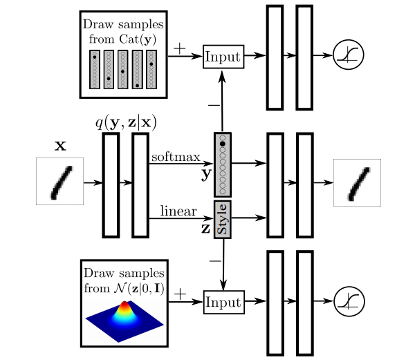
The semi-supervised architecture for adversarial autoencoder is illustrated in the figure above. This is figure 8 from the paper. Let's briefly understand what are adversarial autoencoders in the context of the figure above. There are three different neural interfaces shown in the figure. The central neural network (interface 1) takes the input $\mathbf{x}$ and encodes into it's latent representation $\mathbf{z}$. The encoder also outputs the label $y$ associated with the input. The decoder then takes $\mathbf{z}$ and $y$ and tries to reconstruct back the input $\mathbf{x}$. The encoder-decoder together are termed as autoencoder. The latent representation $\mathbf{z}$ is drawn from a Gaussian distribution. In order to accomplish this, a minimax game is constructed where a second neural network (interface 2) is trained to discriminate between samples coming from the autoencoder interface 1 and those generated from a Gaussian distribution $p(z)$. On the other hand, the encoder tries to generate $\mathbf{z}$ so as to fool the discriminator into believing that the sample came from a Gaussian distribution. This iteration back and forth ultimately results in generator generating samples that the discrimantor and no longer able to separate. Similarly, we would want the label $y$ to come from categorical distribution and reconstruct a similar game for $y$. Let's call this interface 3. The term adversarial stems from the fact that the generator and the discriminator networks are adversary. This is kind of imposing a prior on $\mathbf{z}$ and $y$ and therefore is also termed as adversarial regularization. At the end of the training, the decoder can take a point $\mathbf{z}$ drawn from a Gaussian distribution and a point $y$ drawn from a categorical distribution and generate a sample representative of the data. Thus, the decoder on its own is a generative model. One interesting piece of work showed that if you draw a straight line between the latent representation $\mathbf{z}$ of two sentences and apply the decoder on the points sampled from this line, then the generated sentences show a homotopic transition between the two original sentences. The method of inference used in the paper however was based on variational inference.

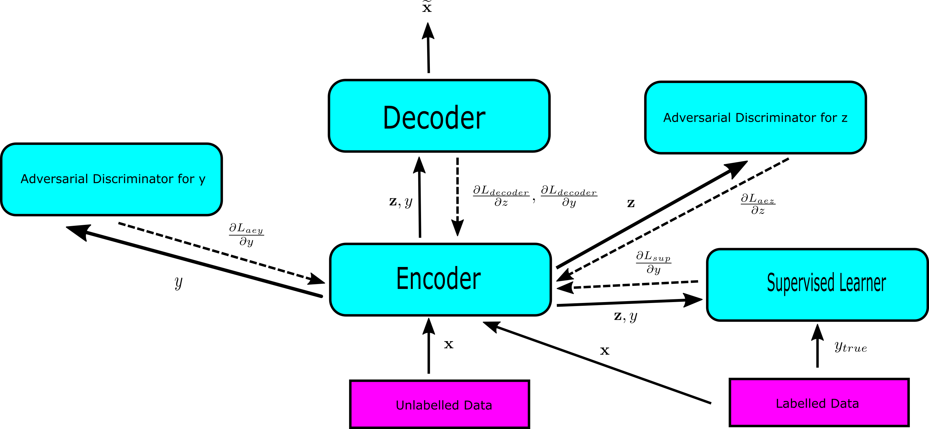
So, in this architecture we have 3 different interfaces synchronously dependent on each other and the entire network is trained end-to-end.

The flow of inputs and gradients is illustrated in the figure above. The objective function $L$ is a sum of 4 different functions $$ \begin{equation} L = L_{decoder} + L_{aez} + L_{aez} + L_{sup} \end{equation} $$ where is $L_{decoder}$ is autoencoder function, $L_{aey}$ and $L_{aez}$ are adversarial functions and $L_{sup}$ is supervised learning loss function. $\mathbf{x}$ is the input, $\mathbf{z}$ is the encoding of the encoder, $y$ is label predicted by encoder, $y_{true}$ is the true label and $\widetilde{x}$ is output of the decoder. Each of the 4 different objective functions are in turn a sum over the data points. Note that when this setup is trained, each interface is synchronously locked for inputs and gradients from other interfaces. In the end-to-end synchronous training, the entire process would be as slow as its slowest unit.

A note on stochastic approximation of gradients

At this juncture, it would be useful take a little detour to understand a related concept. The work horse in deep neural network training has been what is known as stochastic approximation of gradients together with backpropagation described earlier. In brief, the objective function is a sum of many components. Each of these components are in turn sum over many data points. Thus, the gradients are a sum over several terms (objective functions and data points). Each of the terms of this sum can be evaluated and applied independently and in any order! Despite this pronounced stochasticity, the dynamics of the network parameters continue to have a fixed point corresponding to a local minima of the objective function. The value of the objective function in this process will oscillate a bit, but would eventually converge almost surely to a local minima (or a saddle point). It is important to fully understand this in order to appreciate the novelty of gradient based training using mini-batches. Large scale machine learning and the asynchronous network architecture discussed in this post is possible due to this approximation.

Asynchronous architecture

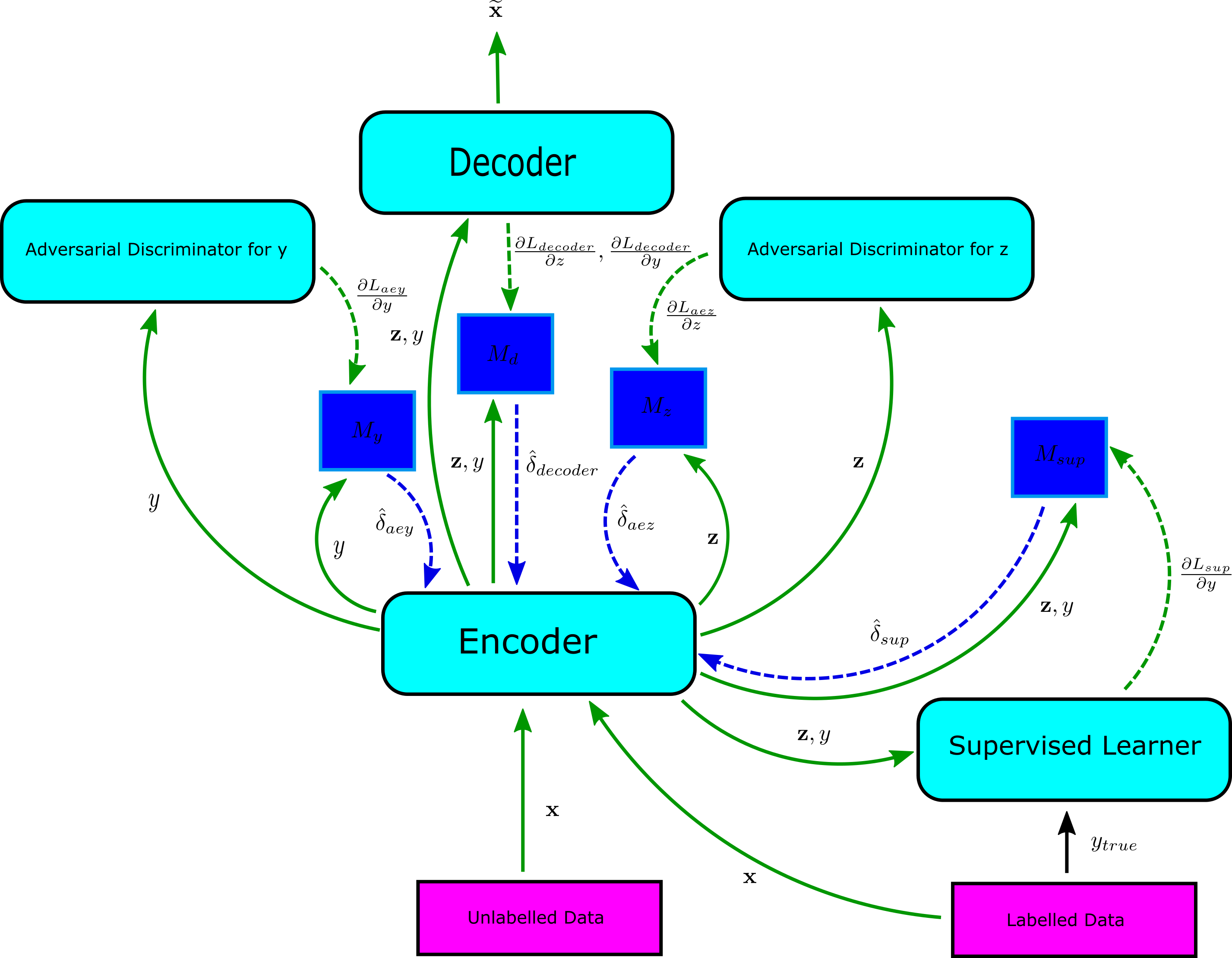
The components of the network for semi-supervised learning using adversarial autoencoders can be decoupled from each other using synthetic gradients. This is illustrated in the figure above. The true information flow is represented by green arrows and synthetic information flow is represented by blue arrows. The inputs are shown by solid arrows and the gradients are shown by dashed arrows. The data $\mathbf{x}$ flows into the encoder that requires gradient information from several upstream modules to update itself. Instead of waiting for the backward flow of gradients, the encoder interrogates about these gradient from 4 different helper networks $M_y$, $M_d$, $M_z$ and $M_{sup}$ shown in blue. These supply the synthetic gradients $\hat{\delta}_{aey}$, $\hat{\delta}_{decoder}$, $\hat{\delta}_{aez}$ and $\hat{\delta}_{sup}$. The true gradients eventually reach these helper network and then these helper networks update their own network parameters. This decoupling allows the unlabelled data to be processed and incorporated into the learning independently of the labelled data. As noted previously, the amount of unlabelled data is many orders of magnitude more than the labeled data. Thus, we would like either to keep the size of mini-batch for the unlabelled data large so as to be able to process a much bigger data stream. Alternatively, we would like to process several mini-batches before we hand over latent codes of $\mathbf{z}$ for downstream processing. Instead, if we decouple and break this synchrony, each of the interfaces can ingest data and update themselves at their own speed. They can independently and asynchronously update themselves using synthetic gradients and inputs.

Various interfaces can of course be composed of many submodules. The submodules can once again be decoupled from each other using synthetic inputs and gradients. The figure above shows the components of the encoder. Our input data is going to be textual, since our motivating example is from the world of advertising. Thus, an embedding layer transforms each of the symbolic language tokens into a real-valued vector space. The embedded input is shown as $\mathbf{x_e}$ in the figure. This embedding transformation itself has to be learned as a part of the training process. The embedded words are then fed into recurrent neural network. In the figure above, we have used a LSTM unit. The LSTM unit receives the synthetic embeddings $\mathbf{\hat{x}_e}$ from the helper network $I_e$. The embedding layer also receives synthetic gradients $\hat{\delta}_{lstm}$ from the helper network $M_{lstm}$. The encoder finally outputs the latent representation $\mathbf{z}$ and the label $y$. The decoder and the supervised learner similarly have such submodules which can possibly be decoupled from each other.

Closing thoughts

An alternative way of thinking about the framework is in terms of adaptive error critic and approximated dynamic programming. The helper networks providing the synthetic gradients are in a way error critic first discussed by Paul Werbos. He is also attributed as one of the individuals who invented the backpropagation. The helper networks approximate the true error by an approximate error and thereby provide the synthetic gradients. Werbos called such networks as critic network and action network with critic network approximating the error and action network providing the control input using this approximated error. The helper network may also be seen as a reinforcement learning controller that outputs appropriate controls in terms of synthetic gradients and gets the rewards of its action when it receives the true gradients.

There have been several alternate lines of work using a randomization approach to approximate gradients using only local information. A recent work has carried such randomization even further by directly incorporating the error from output as a training signal in each layer via a fixed random matrix. The methodology which has been described as direct feedback alignment is similar in spirit to asynchronous teaching signals discussed in this post. The network learns to align itself with the feedback it receives about the objective function. This paradigm has also been termed as learning to learn. See also references [8] and [9]. The biological brain is obviously not using backpropagation for learning due to it's phase locking and non-local nature. We still have to completely understand how learning happens in the real brain and the idea of synthetic gradients is perhaps a practical translation of how a brain-like learning could be mimicked in an industrial situation where the network size is large.

References

[1] Decoupled neural interfaces using synthetic gradients, Max Jaderberg, Wojciech Marian Czarnecki, Simon Osindero, Oriol Vinyals, Alex Graves, Koray Kavukcuoglu, https://arxiv.org/abs/1608.05343, 2016

[2] Automatic differentiation in machine learning: a survey, Atilim Gunes Baydin, Barak A. Pearlmutter, Alexey Andreyevich Radul, Jeffrey Mark Siskind, https://arxiv.org/abs/1502.05767, 2015

[3] Generative Adversarial Networks, Ian J. Goodfellow, Jean Pouget-Abadie, Mehdi Mirza, Bing Xu, David Warde-Farley, Sherjil Ozair, Aaron Courville, Yoshua Bengio, https://arxiv.org/abs/1406.2661, 2014

[4] Adversarial Autoencoders, Alireza Makhzani, Jonathon Shlens, Navdeep Jaitly, Ian Goodfellow, Brendan Frey, http://arxiv.org/abs/1511.05644, 2015

[5] Generating sentences from a continuous space, Samuel R. Bowman, Luke Vilnis, Oriol Vinyals, Andrew M. Dai, Rafal Jozefowicz, Samy Bengio, https://arxiv.org/abs/1511.06349, 2015

[6] Auto-Encoding Variational Bayes, Diederik P Kingma, Max Welling, https://arxiv.org/abs/1312.6114, 2013

[7] Direct Feedback Alignment Provides Learning in Deep Neural Networks, Arild Nøkland, https://arxiv.org/abs/1609.01596, 2016

[8] Random feedback weights support learning in deep neural networks, Timothy P. Lillicrap, Daniel Cownden, Douglas B. Tweed, Colin J. Akerman, https://arxiv.org/abs/1411.0247, 2014

[9] How Important Is Weight Symmetry in Backpropagation?, Qianli Liao, Joel Z. Leibo, Tomaso Poggio, http://arxiv.org/abs/1510.05067, 2016