Beyond Transformers:
Structured State Space Sequence Models

Chetan Nichkawde

January 22, 2024

Sequence modeling has taken centre stage in the world of artificial intelligence with the advent of large language models. However, the cost of training these models and subsequent cost of inference makes it prohibitively difficult for large scale adoption. These models are built upon Transformers-based architectures. A new paradigm is rapidly evolving within the realm of sequence modeling that presents a marked advancement over the Transformer architectures. This new approach demonstrates superior capability compared to Transformers in accurately modeling extensive sequence lengths and contextual dependencies. It exhibits an order of magnitude improvement in computational efficiency during training and inference.

Why do we want to go beyond Transformers?

What makes Transformers great?

The efficacy of self-attention due to its ability to route information densely within a context window, allowing it to model complex data.

What are the challenges with Transformer models?

• Inability to model anything outside of the context window.
• Quadratic complexity and scaling for training and inference with respect to the sequence length.

What makes State Space models great?

• It has linear complexity with respect to the sequence length during the training time which can easily be parallelized using parallel scans.
• Many times faster during inference. It can do inference in constant time using the current state compared to Transformers which requires computation of self-attention over the entire context.
• They can easily model very long range context and have been shown to model a context length of about 1 million tokens. The Transformers cannot model long context due to quadratic scaling with respect to the sequence length.
• They can do inferences on sequences of any length and longer than the longest sequence in the training data.

The table below shows the results on Long Range Arena benchmark which has a set of tasks on data with long sequences.

Long Range Arena Benchmark

Model	ListOps	Text	Retrieval	sCIFAR	Pathfinder	Path-X	Avg
Transformer	36.37	64.27	57.46	42.44	71.40	✕	53.66
Reformer	37.27	56.10	53.40	38.07	68.50	✕	50.56
BigBird	36.05	64.02	59.29	40.83	74.87	✕	54.17
Linear Trans.	16.13	65.90	53.09	42.34	75.30	✕	50.46
Performer	18.01	65.40	53.82	42.77	77.05	✕	51.18
FNet	35.33	65.11	59.61	38.67	77.80	✕	54.42
Nystromformer	37.15	65.52	79.56	41.58	70.94	✕	57.46
Luna-256	37.25	64.57	79.29	47.38	77.72	✕	59.37
LRU	60.2	89.4	89.9	89.0	95.1	94.2	86.3

We can see that the results for Linear Recurrent Unit (LRU) discussed in this article far exceed all the Transformers based models. Furthermore, the state space based models are 5 to 10 times faster on inference speed while requiring only 10% of the memory compared to Transformers. The longest context is about 16000 for the task Path-X. All of the Transformer based models are not able to solve this task while LRU has an accuracy of about 94%. The purpose of this article is to develop a foundational level understanding on how structured state space sequence models work in efficiently modeling long sequences.

The quintessential spring-mass-damper system

We start our discussion with spring-mass-damper system which is one of the most widely studied systems in classical mechanics and dynamics. The ideas from this template system have already been applied to various fields in science and engineering. For instance, if you want to understand the flight stability characteristics of a rocket flying in the atmosphere carrying a large amount of liquid fuel, you can apply a similar analysis performed for the rocket system linearized around an equilibrium point. We will see later that the linear dynamical systems also form the backbone of the futuristic sequence models which alleviates the challenges with Transformer models while offering the same level of modeling fidelity.

Figure 1: A spring mass damper system with external forcing.

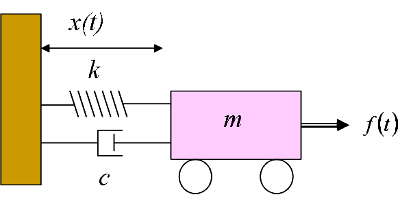
Shown above is an object with mass $$m$$ attached to a wall with spring with a spring constant $$k$$ and a damper with damping coefficient $$c$$. The displacement of the object is represented by $$x(t)$$. The object is forced by an external time dependent force $$f(t)$$. The $$f(t)$$ we will later see is equivalent to our sequential data. The spring $$k$$ is a potential energy store that is converted into kinetic energy of the object in an oscillatory fashion. The damper $$c$$ usually dissipates the energy when $$c$$ is positive. A strong damping can quickly dissipate the energy leading the object coming to almost rest (remember vanishing gradients?!). However, $$c$$ can also be negative in which case the damper can actually absorb more energy from the environment and add it to the system eventually leading to explosion (remember exploding gradients?!). We will see later these dynamic stability characteristics have a deep connection with the modeling fidelity of our sequence model and we want to create inductive biases in the model formulation such that a similar linear dynamical system like the above has good dynamic characteristics that facilitate learning.

The vanishing and exploding gradients can also be understood in terms of the stability of the dynamics of backpropagation. Here we are motivated by the need to find efficient parametrization to ensure just the right kind of dynamics during the forward pass.

Let us formulate the equations of motion for this system using the Newton's second law of motion: F = ma where the force $$F$$ is F = -c\dot{x}-kx The spring-mass-damper system also has a time-dependent driving force $$f(t)$$ which represents the input to the system and our sequential data. Putting it all together: m\ddot{x} = -c\dot{x}-kx+f(t) Now we express this equation in state-space form. Let $$x_1 = x$$ and $$x_2 = \dot{x}$$. Rewriting above: \begin{array}{l} \dot{x}_1 = x_2 \\ \dot{x}_2 = -\frac{c}{m}x_2 - \frac{k}{m}x_1 + \frac{1}{m}f(t) \end{array} Expressing it in matrix form: \dot{\mathbf{X}} = A\mathbf{X} + B\mathbf{U}(t) \qquad (1) where \mathbf{X} = \begin{bmatrix} x_1 \\ x_2 \end{bmatrix}, \quad \mathbf{U} = \begin{bmatrix} 0 \\ f(t) \end{bmatrix} A = \begin{bmatrix} 0 & 1 \\ -\frac{k}{m} & -\frac{c}{m} \end{bmatrix}, \quad B = \begin{bmatrix} 0 \\ \frac{1}{m} \end{bmatrix}

The dynamical stability characteristics of any system expressed in the above form, also known as state-space form, can be completely understood by inspecting the eigenvalues of the matrix $$A$$. We want to have a positive damping to ensure stability. We can easily extend the above analysis to a multi-dimensional system.

We want the system to be marginally damped but not overdamped from a deep learning perspective.

Let's work out the formula for eigenvalues. The characteristic equation is given by: m\lambda^2 + c\lambda + k = 0 The roots (eigenvalues) are given by: \lambda_{1,2} = \frac{-c \pm \sqrt{c^2 - 4mk}}{2m} When the discriminant $$\Delta = c^2 - 4mk$$ is negative, the eigenvalues become complex conjugates. Let's consider the case where the discriminant is negative: The natural frequency $$\omega_n$$ of the system defined as: \omega_n = \sqrt{\frac{k}{m}} The eigenvalues can then be expressed in terms of $$\omega_n$$ as: \lambda_{1,2} = \frac{-c}{2m} \pm j\omega_d where $$j$$ is the imaginary unit, and $$\omega_d$$ is the damped natural frequency given by: \omega_d = \sqrt{\omega_n^2 - \frac{c^2}{4m^2}}

It is always possible to apply a coordinate transform such that the state transition matrix $$A$$ is diagonalized with the eigenvalues as the diagonal entries. Thus, we can get a decoupled set of equations of the following form: \frac{dx(t)}{dt} = \lambda x(t) where $$\lambda$$ is the eigenvalue. To solve this ODE, we can separate variables and integrate: \int \frac{dx}{x} = \lambda \int dt Integrating both sides gives: \ln(x) = \lambda t + C where $$C$$ is the constant of integration. Taking the exponential of both sides: x(t) = e^{\lambda t + C} x(t) = e^{C} e^{\lambda t} We can rewrite the above as: x(t) = x_0e^{\lambda t} \qquad (2) where $$x_0$$ is the initial state.

Since the real part of $$\lambda$$ is $$\frac{-c}{2m}$$, it is easy to see from Equation (2) why we need a positive damping $$c$$ for the system to be stable. The exponential term will blow up as time progresses for a negative value of $$c$$ making the system unstable. We will revisit this equation in the Section Designing linear recurrent unit.

It is important to note that the system represented by Equation (1) is linear. The matrices $$A$$ and $$B$$ do not depend on the state $$x$$ and the input $$f(t)$$. At this point, it would be good to introduce another equation for the output $$y$$. y(t) = C\mathbf{X} \qquad (3) The output for the autoregressive model is the future value in time of $$f(t+1)$$. It would be the next token $$u_{k+1}$$ for a sequence model.

The data in the real world is always discrete especially if you are trying to model discrete sequences like language, protein or DNA. The continuous time ordinary differential Equation (1) can easily be discretized using methods like Zero-Order Hold or Bilinear transform. We will skip the details of discretization but a similar stability analysis can be performed for a discrete time system as well.

Introducing Recurrent Neural Network

The model represented by Equation (1) is a special form of recurrent neural network (RNN). A general recurrent neural network is fully nonlinear and does not have nice a state-space form. Nonlinearities are also important as they are needed for the modeling fidelity. The nonlinear parts are added as projection layers before and after the linear state-space components as will see later. The recurrent neural network offers a significant advantage over Transformers when it comes to the inference speed. Have a look at Equation (3). What do you see? The output can easily be computed in constant time using the value of current state $$\mathbf{X}$$. Transformers require $$\mathcal{O}(L^2)$$ time to compute the output where $$L$$ is the length of the sequence. Furthermore, the Transformers cannot process sequences longer than the maximum limit defined by its architecture. The RNN can process sequences of any length including sequences longer than the longest sequence it saw during the training.

The difficulty of training a nonlinear RNN

A nonlinear recurrent neural network however is difficult to train due to vanishing or exploding gradient problem. The dynamics are either too stable or unstable and the information signals either vanish or explode as we traverse across the sequence. Such instabilities can be understood from the linearized version of the nonlinear RNN and using an analysis similar to the discussion in the Section The spring mass damper system.

Figure 2: Bifurcation diagram for a single node RNN.

Additionally, these instabilities can also arise in nonlinear systems due to a phenomenon known as bifurcation where there is a discontinuous jump in the asymptotic state due to very small changes in the parameter. The figure above is taken from a classical paper listed as Ref . Figure 2 shows the asymptotic values of neuron state $$x$$ in a single neuron RNN as we vary the bias parameter $$b$$. The figure shows 3 distinct parameter regimes: 1) $$ b < b_2 $$ 2) $$ b_2 < b < b_1 $$ 3) $$ b > b_1 $$. There is only one asymptotic state which varies smoothly as $$b$$ changes for the regime 1 with $$ b < b_2 $$. However, the regime 2 with $$ b_2 < b < b_1 $$ is very interesting. There are 3 possible asymptotic states in this regime with 2 of them being stable while the third one shown as dashed line is unstable. The neuron can end up in any of these states depending on the initial condition or the amount of perturbation from its current state. There is a basin of attraction for each of the 2 stable state. What does this mean in terms of training the RNN? It means the RNN could end up losing all its learning as $$ b $$ crosses the value $$ b_2 $$ because the RNN may jump from one stable state to another stable state. The regime 3 is even more catastrophic as the the RNN will surely undergo a discontinuous jump as $$ b $$ crosses the value of $$ b_1 $$ and as a result forget all its prior learnings. This is an example of subcritical Hopf bifurcation.

Thus, the nonlinear RNNs do not perform as well as Transformers that densely route information over the token graph using the self-attention mechanism. They cannot model long sequences like a DNA. Transformers however have a significant disadvantage due to their quadratic complexity and once again cannot be used to model long sequences.

This sets the motivation for this article. We want to design a neural network that scales as $$\mathcal{O}(L)$$ during training and can do inference in constant time where $$L$$ is the length of the sequence and $$L$$ can be very long up to the order of 1 million tokens. We want deep information propagation capability that can transmit the signal for very long sequence lengths.

Koopman operator: Linearized dynamics in a nonlinear function space

We saw that state-space models represented as linear system allow us to explicitly design for its stability characteristics by placing the real part of eigenvalues of the state transition matrix $$A$$ in the left half of the complex plane. Furthermore, we will see later that a diagonalized version $$A$$ can also help parallelize computations using parallel scans. Clearly, it's advantageous to have the dynamics part in a linear form. We can separate the nonlinear part of the network that imparts modeling fidelity from the linearized dynamics using the Koopman operator theory. The Koopman operator theory says that it is possible to find an appropriate coordinate transform where the strongly nonlinear dynamics is approximately linear. Stated simply, we can represent these nonlinear transforms using a feedforward multi-layer perceptron (MLP) and apply the methods of linear state-space system to the output. The nonlinear transform and the linearized dynamics are learned end-to-end using deep learning.

The idea is similar to kernel functions in Support Vector Machines which finds linearly separable inner product space using Kernel functions. The Gaussian kernel projects the input into an infinite dimensional space similar to the Koopman eigenfunctions.

Designing the linear recurrent block

Let us now get to the core of this article. The core unit that processes the sequence will be called the Linear Recurrent Unit (LRU). Most of the presentation in this section builds upon the work from Ref . There are other work on structured state space models that develops the same idea of interleaving nonlinear MLP blocks with linear state-space models and differ in the way they structure and initialize $$A$$ and $$B$$ matrices. These include S4, S5, and, Mamba.

Lets once again rewrite the linear recurrence relationship in discrete form and from here on we will use $$x_k$$ to represent the value of state and $$u_k$$ to represent the discrete input at time step $$k$$ x_{k} = Ax_{k-1} + Bu_k The above recurrence relationship can easily be unrolled as follows: x_0 = Bu_0, \quad x_1 = ABu_0 + Bu_1, \quad x_2 = A^2Bu_0 + ABu_1 + B u_2, \implies x_k = \sum_{j=0}^{k-1} A^jBu_{k-j} \qquad (4)

Diagonalizing $$A$$

Note that if $$A$$ in above relationship is diagonal then $$A^j$$ can be easily computed. Furthermore, linear RNN layers with a diagonal structure enable efficient parallel unrolling of the recurrent process through parallel scans, leading to significantly faster training speeds. We can make use of the fact that every non-diagonal matrix is diagonalizable to apply the eigenvectors based coordinate transform to diagonalize $$A$$ resulting in a diagonal matrix with potentially complex valued entries. Thus, the Equation (4) can be expressed as follows: x_k = \sum_{j=0}^{k-1} \Lambda^j B u_{k-j} \qquad (5) where $$\Lambda$$ is a diagonal matrix with eigenvalues of $$A$$ as its diagonal entries.

Stable exponential parameterization

It is easy to see that the norm of component $$j$$ of $$x$$ at timestamp $$k$$ evolves such that $$x_{k,j} := \mathcal{O}(\lambda_j^k)$$ where $$\lambda_j$$ is the diagonal entry in the $$j^{th}$$ row of the diagonal matrix $$\Lambda$$ discussed in the Equation (5) and it is the $$j^{th}$$ eigenvalue of $$A$$. We can use exponential parameterization of $$\lambda_j = e^{\nu_j+i\theta_j}$$ discussed in the next section to bring it in same form as Equation (2) and thus $$x_{k,j} := \mathcal{O}(e^{-k\nu_j}e^{i\theta_j})$$. Therefore, a sufficient condition for $$x_{k,j}$$ to not explode and ensure stability is $$\nu_j > 0$$ for all $$j$$.

Figure 3: The input for the sequence $$aa$$. The sequence $$ab$$ will have the second pulse of the opposite sign.

Figure 4: The response of the system with sequence input $$aa$$ for low damping, highly damped, and, negatively damped systems.

Figure 5: The response of the system with sequence input $$ab$$ for low damping, highly damped, and, negatively damped systems.

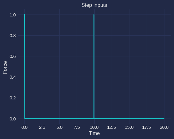
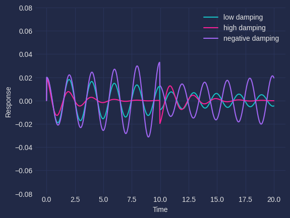
It is also important to note that if $$\nu_j$$ is very large then $$x_{k,j}$$ will vanish which is an impediment in modeling long sequences where $$k$$ is very large. The information propagation capacity and stability of dynamics in the forward pass is demonstrated in Figures (4) and (5). Let's model two sequences each with 2 tokens. The first sequence is $$aa$$ and the second sequence is $$ab$$. $$a$$ and $$b$$ tokens have 1-dimensional embeddings of 1.0 and -1.0 respectively. These inputs are fed to the system at an interval of 10 seconds. The inputs for $$aa$$ is shown in Figure (3). The input for $$ab$$ will be similar with the opposite sign of the pulse at $$10^{th}$$ second. We consider the response of 3 different systems with -- 1) low damping ($$\nu_j > 0$$) 2) high damping ($$\nu_j \gg 0$$) 3) negative damping ($$\nu_j < 0$$) for these two sequences. The information for the first token $$a$$ attenuates quickly for the highly damped system and the final state is indistinguishable for the two sequences. However, for an appropriately damped system shown in green the final state differs for the two sequences representing successful information propagation. The amplitude for the negative damped case will gradually grow unbounded for both the sequences making the network unstable. Thus, we need to set the right inductive bias in the model for it to be appropriately damped in order to foster long range information propagation capability.

We enforce the condition above making use of Lemma 3.2 in Ref which is given as follows: Let $$u_1,u_2$$ be independent uniform random variables on the interval $$[0,1]$$. Let $$0\le r_{\min}\le r_{\max}\le1$$. Compute $$\nu = -\frac{1}{2}\log\left(u_1(r_{\max}^2-r_{\min}^2)+r_{\min}^2\right)$$ and $$\theta = 2\pi u_2 $$. Then $$\exp(-\nu+i\theta)$$ is uniformly distributed on the ring in complex plane $$\mathbb{C}$$ between circles of radii $$r_{\min}$$ and $$r_{\max}$$.

The Glorot initialization naturally places the eigenvalues within the unit circle in the complex plane.

Figure 6: Exponential initialization of eigenvalues within a ring.

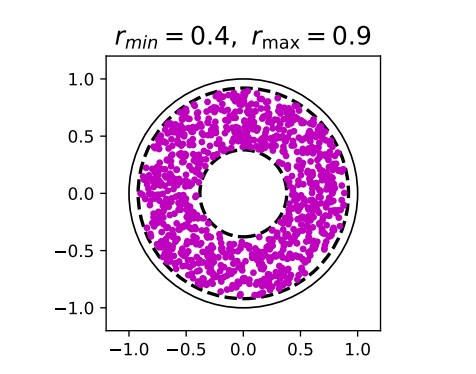
This is shown in the above figure with $$r_{min} = 0.4$$ and $$r_{max} = 0.9$$. This suggests a natural parameterization for $$A$$ as $$\Lambda = \text{diag}(\exp(-\nu + i \theta))$$ with $$\nu$$ and $$\theta$$ as the learnable parameters.

Exponential parameterization only solves half of the problem by keeping the eigenvalues confined within a ring inside the unit circle and therefore bounded. We also need to ensure the stability of the dynamics discussed in spring-mass-damper example by having a positive damping. We need to ensure that $$\nu > 0$$ (this ensures positive damping similar to $$c > 0$$ in the spring-mass-damper system). This is easy to do if we use another positive nonlinearity in the form of exponential: $$\lambda_j:=\exp(-\exp(\nu_j^{\log})+i\theta_j)$$, where $$ \nu^{\log}_j $$ is the parameter that is optimized. We can see from Equation (5) having the term $$\Lambda^j$$ that we need to initialize the eigenvalue closer to the unit disk by making $$r_{min}$$ closer to 1 ($$\lambda_j^k \approx 0$$ when $$\lambda_j \ll 1$$) for deep information propagation and model long range interactions.

Designing the transient dynamics through small phase

Additionally, in the studies in Ref it was also found that the LRU has to be initialized with a small phase $$\theta_j \approx [0,\pi/50]$$ to be able to do well on the most difficult task of Path-X.

Path-X positive sample.

Path-X negative sample.

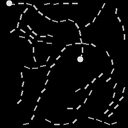
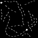
The figure above shows the positive and negative samples for the Path-X task. The image consists of 16000 pixels which are fed sequentially to the model. The task is to ascertain if the two white dots are connected by a path. Unconstrained initialization between $$[0,2\pi]$$ can result in high frequency dynamics with large number of oscillations (see Figure 4 in Ref ). The presence of high frequency components makes the system quickly settle into its autonomous modes and the memory of the input is lost. We would like the dynamics to stay transient and driven by the inputs (see Ref ).

The full neural network architecture

Figure 7: The complete architecture for LRU. This is Figure 1 from Ref .

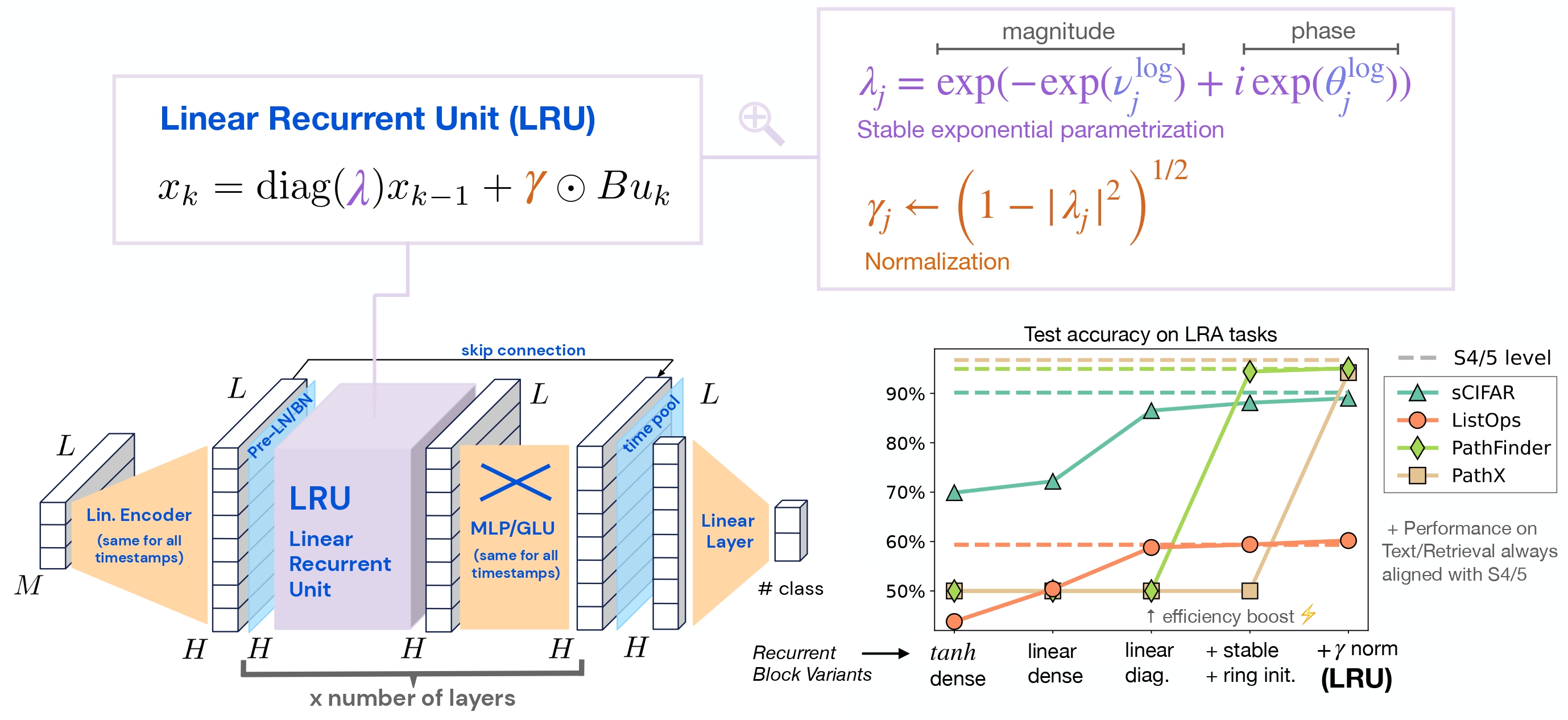
The complete architecture for the entire network is shown in Figure (7). The $$M$$ dimensional input of length $$L$$ is projected into a dimension $$H$$ (see Section Koopman operator). The layer normalization or batch normalization is applied before passing it on to LRU. The LRU outputs are further processed using GLU and skip connection.

Why use linear recurrent block?

Given all the discussions so far, let us summarize as to why we want to use a linear recurrent block.

• Transformers are inefficient with $$\mathcal{O}(L^2)$$ complexity during training and inference.
• RNNs have $$\mathcal{O}(L)$$ complexity during training and can do inference in constant time.
• A nonlinear RNN is difficult to train due to bifurcations encountered during training (see Section The difficulty of training RNN).
• The nonlinear RNN requires unrolling one time-step at a time and therefore cannot be parallelized.
• The nonlinearities added before the linear recurrent blocks are sufficient to ensure modeling fidelity and afford universal computation according to Koopman operator theory (see Section Koopman Operator).
• The linear recurrence can be computed in one single step by recursively expressing the state over the time range as a function of input. It is possible to relate the final state to the input sequence with a simple equation without the need to compute the intermediate state (see Equation (4) in Section Designing Linear Recurrent Unit).
• Every non-diagonal state space model can be diagonalized with a reparametrization with potentially complex entries. The diagonalized $$A$$ offers additional computational efficiency using parallel scans (see Section Diagaonalizing $$A$$).
• We can design the stability characteristics of the linear system to be appropriately stable and ensure stability during training giving us the ability to model long sequences with fast training and inference (see Section Stable exponential parametrization).
• Keeping the imaginary part of the eigenvalue $$\theta$$ also known as phase is necessary to ensure that oscillations are driven by inputs and hence encode the information about the input (see Section Designing the transient dynamics).

Further thoughts: Resurrecting nonlinear recurrent units on hardware

We saw in the Section Designing the transient dynamics that it was necessary to keep the phase small (imaginary part of the eigenvalue) to solve the most difficult task of Path-X in the long range arena benchmark.

Thus, the information and memory about the sequence is stored in the transient dynamics of the linear dynamical system that we designed. We designed these transients to be stable by creating an inductive bias that places the real part of the eigenvalue in the left of the complex plane. The transients will blow up if the system is unstable (see Figure (4) and (5)). The linear state space models also afforded fast computation through the use of Equation (5) and parallel scans. It is possible to reap all of the above benefits through the use of certain class of nonlinear dynamical systems that can also be implemented on hardwares that are fast, energy efficient, and, have very high bandwidth. These systems are both unstable and stable at the same time. They are composed of multiple modes many of which are unstable. However, their oscillations are still bounded due to the presence of nonlinearities. They have tremendous information processing capacity because they are repositories of rich dynamical patterns in the form of transients that can serve as an effective kernel. A photonics based hardware can process million words per second. There is also no need to train these nonlinear recurrent units on hardware. The only trainable components would be preprocessing and post processing components placed before and after these nonlinear recurrent unit blocks.